To be honest, we normally don't want our robot to tell us where it is - we want to tell where it should be. How does we achieve this? Imagine you have a GPS device and want to move to 22°13'27.8"N 22°06'55.7"E. The GPS device only tells you your position, just the coordinates, no map. You are for sure able to get to the goal position by moving in a random direction and comparing the coordinates on your device with the goal coordinates, but this would be quite inefficient. If we tell our robot to move to the goal pose (0.5, 0.1) with a rotation of 0.75, it could start moving its motors in a random direction and compare how much the current pose of the end-effector differs from the goal pose.

Try it out yourself! Can you move the end-effector to (0,0) with a rotation of 0? The current pose is displayed at the bottom of the simulation.

However, it would be much better if we could just compute the configuration - the joint angles - the robot will have at the goal pose and move the joints straight to this configuration.

In other words, we try to find a formula which takes a pose as an input and outputs the configuration q of the robot. In forwards kinematics we developed a formula which takes the configuration as an input and outputs the pose. We therefore call this problem - you might have guessed it - inverse kinematics or IK for short.

Unfortunately there is no one size fits all solution. Depending on the robot, the complexity of this problem varies significantly and there are different strategies to solve it. Two major approaches are algebraic and geometric inverse kinematics.

Algebraic Inverse Kinematics

For algebraic inverse kinematics, an equation system is set up and solved. For our planar robot we could use the three equations for the forwards kinematics and solve them for $q_0$, $q_1$ and $q_2$. These equation are

$\phi_{O,ee} = q_0+q_1+q_2$

$x_{O,ee} = l_0 \cdot cos(q_0) + l_1 \cdot cos(q_0+q_1) + l_2 \cdot cos(q_0+q_1+q_2)$

$y_{O,ee} = l_0 \cdot sin(q_0) + l_1 \cdot sin(q_0+q_1) + l_2 \cdot sin(q_0+q_1+q_2)$

where $l_0$, $l_1$ and $l_2$ are the lengths of the links. With a good mathematical software solving these equations would be a matter of plugging in the formulas and waiting for a solution. However, in this article I want to show you a goemetric approach.

Geometric Inverse Kinematics

As the name of this approach suggests, we are going to use a lot of trigonometry. TO be prepared for the next sections, it is helpful to have the definitions of sine, cosine and tangent in mind. We also use the Pythagorean theorem and the law of cosines.

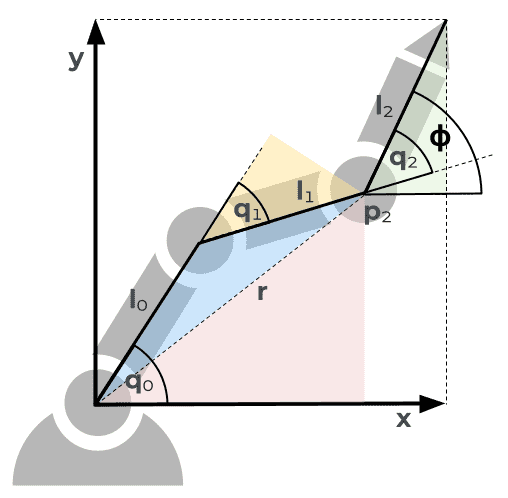
In the following image you see our robot with an arbitrary pose. Given x, y and $\phi$, we want to compute the three joint angles $q_0$, $q_1$ and $q_2$. I marked four triangles in the image, a green, red, yellow, and blue one. Let's look what we know about these triangles.

Green triangle

We already know a lot about the green triangle. It has a right angle at the bottom right, the bottom left is equal to $\phi$, its hypotenuse is equal to the length of the end-effector $l_2$ and the corner at the top has the position (x,y). With this information we can compute the position of $p_2$, the center of the joint connected to the end-effector. With the definition of sine and cosine, we can compute the length of the bottom side of the rectangle with $l_2 \cdot sin(\phi)$ and the right side of the triangle with $l_2 \cdot cos(\phi)$. The point $p_2$ is therefore defined as

Red triangle

The red triangle has a right angle at the bottom right corner. We can therefore use the Pythagorean theorem to compute the hypotenuse r by using the x- and y- coordinate of $p_2$.

$r^2 = x'^2 + y'^2$

Furthermore, we can compute the the angle at the bottom left corner with $atan\Big(\frac{x'}{y'}\Big)$

Blue triangle

Now things get more complicated! The blue triangle has no right angle. We use thefore the Law of cosines $a^2=b^2+c^2-2bc\cos\alpha$ where a, b and c are the sides of the triangle and $\alpha$ is the angle between the sides b and c. In our triangle, $a = r$, $b = l_0$, $c = l_1$ and $\alpha = \pi - q_1$. By rearranging the formula and plugging in the equation for $r^2$ from the red triangle, we are able to compute the angle of the second joint $q_1$.

$q_1 = acos\Big(\frac{x'^2 + y'^2 - l_0^2 - l_1^2}{2l_0l_1}\Big)$

Yellow triangle

The yellow triangle has a right angle at the top. We therefore know, that the side right to the top angle has the length $l_1 \cdot cos(q_1)$ and the side left to the top angle has the length $l_1 \cdot sin(q_1)$

Blue-yellow triangle

The angle of the first joint $q_0$ is the sum of the bottom left angles of the blue and the red triangle. We already computed this angle for the red triangle. The angle for the blue triangle can be computed by looking at the triangle consisting of the blue and the yellow triangle. It has a right angle at the top. The angle at the bottom left is therefore $-atan\Big(\frac{l_1 \cdot sin(q_1)}{l_0 + l_1 \cdot cos(q_1)}\Big)$. We can compute $q_0$ with

$q_0 = atan\Big(\frac{x'}{y'}\Big) - atan\Big(\frac{l_1 \cdot sin(q_1)}{l_0 + l_1 \cdot cos(q_1)}\Big)$

The only angle missing is now $q_2$. We can compute it with $q_2 = \phi - q_1 - q_0$.

Seeing it in action

In the interactive demo below, you can see the inverse kinematics in action. With the sliders on top you can modify x, y and $\phi$. At the bottom you see the values for the three joint angles. Whenever the values for x, y or $\phi$ are changed, the configuration is computed with the formulas we just derived. The configuration is then used to draw the robot.